Source Camera Identification for Forensics [FREE COURSE CONTENT]

In this excerpt from our Digital Video Forensics online course by Dr Raahat Singh we will deal with the complex and interesting topic of Pattern Noise Based Source Camera Identification - if you have a piece of video evidence in your investigation, this knowledge might be very useful, so dive in!

To use pattern noise as a characteristic for sensor fingerprinting, the noise component must first be extracted. Ideally, pattern noise must be extracted from a uniformly lit scene before any non-linear operation is performed on it (which means that the image must essentially be ‘raw’). In a real-life forensic scenario, the analyst does not have access to this raw sensor data that can facilitate extraction of noise characteristics. So, in absence of any direct method of noise extraction, indirect methods are used to estimate the noise component.

PRNU Estimation and Device Linking

The following steps explain the source camera identification process in detail. For the sake of simplicity, we will refer to pattern noise as PRNU.

Step 1 – Estimation of Reference PRNU: The easiest way to calculate an approximation of PRNU for a particular camera (which is referred to as reference PRNU) is to average multiple images captured by the same camera. Ideally, it is suggested that for the computation of reference pattern noise, one must use frames of a flat-field video (with no scene content and an approximately uniform illumination, such as pictures of a wall or cloudless sky) rather than images of natural scenes. Having said that, in case acquisition of a flat-field video is not possible or feasible, frames of any video (recorded by the same device) can be used to estimate PRNU just as well.

When the frames of the video being used for noise estimation exhibit a lot of scene details, frame averaging becomes a time-intensive operation. So, to speed up the process, we first remove the scene content using a denoising filter and then average the noise residuals instead. These steps are explained below.

Step 1.1 – Calculation of Noise Residue: Every frame is first denoised using an appropriate denoising filter (Equation 2.1). The denoised frames are then subtracted from the original frames to obtain noise residue (Equation 2.2).

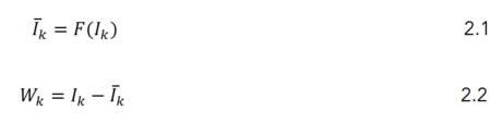
Here, F denotes the denoising filter, I_k denotes the k^th frame of the video and Ī_k is the denoised version of this frame; W_k denotes the noise residue for the k^thframe. The choice for the denoising filter remains wide open; the only consideration is that the noise residue must contain the needed amount of noise components. The amount of noise that survives denoising generally depends on the characteristics of the frame contents. Therefore, the denoising filter must be chosen in a manner that accommodates the needs of the frames under consideration. For instance, a wavelet-based denoising filter generates desirable results in most cases but may sometimes lead to over-smoothing, in which case, a relatively simpler median filter would be a better alternative.

Step 1.2 – Averaging Noise Residue to Calculate PRNU: Once noise residue is obtained for every frame, reference PRNU (N_ref) can be estimated for a set of N frames using Equation 2.3. 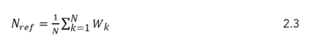Step 2– Estimation of Test PRNU: Test PRNU refers to the pattern noise extracted from the video whose origin needs to be determined. It is calculated in the same manner as reference PRNU; every frame of the video is first denoised using an appropriate filter (the same filter used during the estimation of reference PRNU), followed by computation of noise residue, which is then used to estimate test PRNU (N_test).

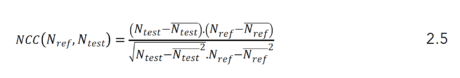
Step 3– Calculation of Correlation Between Reference and Test PRNU: In order to determine if the given video was generated by a particular camera, we need to find the degree of similarity between the noise patterns of the given video and those of the camera. This is done by calculating the correlation between reference PRNU and test PRNU using the standard formula:

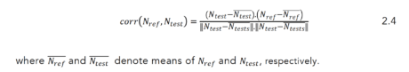
If the correlation thus obtained is above a pre-determined threshold, we can confirm that the video in question was captured by the camera under consideration. In case the given video is to be linked to one of several available cameras, the camera whose reference PRNU is most correlated with the test PRNU is determined to be the source camera. Note that in this case too, a threshold is still required because it is not necessary for any one of the given cameras to be the source camera. For instance, if three cameras generate correlations .36, .21, and .43 with the test PRNU, then camera 3 is not necessarily the source device because the correlation value is still too low, even if it is the highest amongst the three.

Experiment I: Visual Appearance of PRNU Patterns: This simple experiment* will help the reader visualize what noise residue and PRNU patterns look like.

We will conduct the experiment on a standard test video ‘fuji_2800_outdoor(2)’, from the SULFA Video Forensics Library. Two sample frames from this video are presented in Figure 2.9.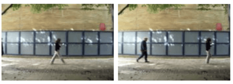

Figure 2.9 Sample frames from the test video ‘fuji_2800_outdoor(2)’ [Video Courtesy of SULFA].

The first step is to calculate noise residue for all the frames of this video, which requires the assistance of a denoising filter; we use two-dimensional median filter. Note that for the sake of simplicity, we will work with grayscale test frames. (Another way to reduce significant computational overhead is to work with only one of the three color channels of an RGB frame.)

Noise residue for the sample video is computed using Equations 2.1 and 2.2; it appears something like this:

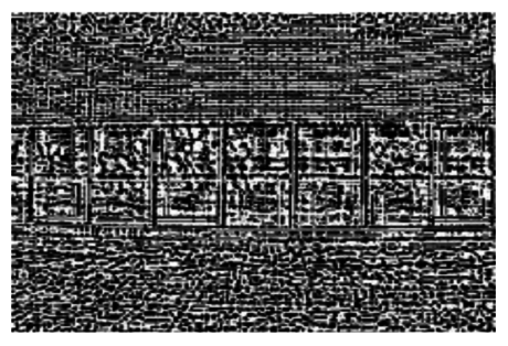Figure 2.10 Noise residue for a sequence of frames.

We can estimate PRNU by averaging the noise residue over multiple frames (the more frames the better) using Equation 2.3 (Figure 2.11).

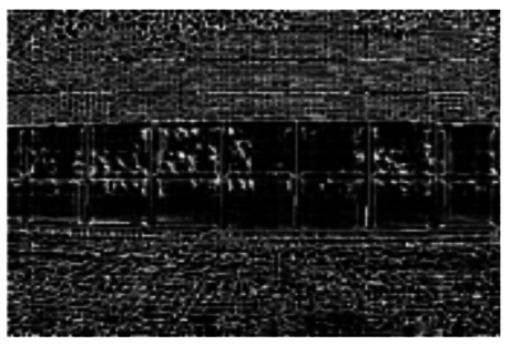
Figure 2.11 Average noise residue (aka PRNU) for a series of frames.

This pattern is then treated as reference PRNU for a particular recording device.

In the next experiment, we will examine the unique nature of PRNU by estimating noise patterns from two sample videos, which depict visually similar scenes but have been recorded using different cameras.

Experiment II: Verification of the Unique Nature of PRNU Patterns: We consider two sample videos, ‘can_220_hallway(3).mov’ and ‘fuji_2800_man(2).avi’ (available from the SULFA Library, and for download here: https://www.dropbox.com/sh/dhzuebt4494ovxa/AADK5mYRdDoJHlEpLXwsDjSDa?dl=0), which depict similar scene contents (Figure 2.12).

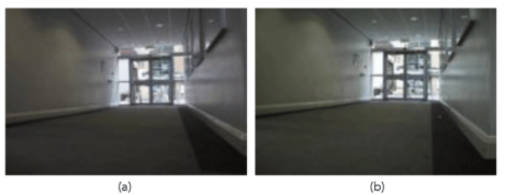
Figure 2.12 (a) represents a sample frame from ‘can_220_hallway(3).mov’ whereas (b) represents a sample frame from ‘fuji_2800_man(2).avi’. [Videos Courtesy of SULFA].

We estimate PRNU for each of these videos; the resultant patterns are presented in Figure 2.13.

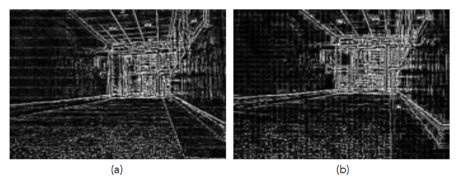
Figure 2.13 (a) represents the PRNU pattern for the video ‘can_220_hallway(3).mov’ whereas (b) represents the PRNU pattern for the video ‘fuji_2800_man(2).avi’.

We can observe from Figure 2.11 that the noise patterns for the two test videos appear quite dissimilar, despite the fact that the videos themselves exhibit visually similar contents (the variations in the patterns are most conspicuous in those regions of the frames that contain the least amount of scene details, such as the walls and the floor). This unique nature of PRNU is the primary reason why it is referred to as the fingerprint of a recording device.

Limitations of PRNU-Based SCI

The PRNU-based camera and sensor fingerprinting method discussed above has been shown to be quite efficient in the literature, but it suffers from a significant drawback, which is that PRNU is highly sensitive to synchronization. A slight geometric transformation, such as scaling, rotation, or cropping on the frames of the video in question, causes desynchronization, which leads to inaccurate detection. PRNU calculations are also unreliable in the presence of compression artifacts.

These limitations can be overcome in two ways: we can either compute normalized correlation coefficient instead of simply correlating test and reference PRNU, or we can modify the noise pattern estimation process.

Normalized Correlation Coefficient

Normalized Correlation Coefficient (NCC) helps neutralize the effects of mild geometric transformations, and can be calculated using Equation 2.5.

Modified Noise Pattern Estimation: SPN Based Analysis

By modifying the noise pattern estimation process, source camera identification techniques can be made more robust. More specifically, instead of PRNU, we suggest working with Sensor Pattern Noise (SPN).

Steps for computation of reference and test SPN are the same as those outlined in Equations 2.1 and 2.2 described above, modifications will be done to Equation 2.3, which now becomes:

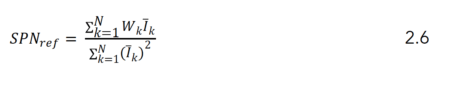
where, I_k denotes the k^th frame of the video and Ī_k is the denoised version of this frame; W_k denotes the noise residue for the k^th frame.

Test SPN (SPN_test) is also calculated in a similar manner. (Correlation and NCC between reference and test SPN can then be calculated using Equations 2.4 and 2.5, but with reference and test SPN rather than PRNU.)

Figures 2.14, 2.15, and 2.16 illustrate sample frames from a test video ‘can_220_street(1).mov’ and the SPN estimated from the frames of this video.

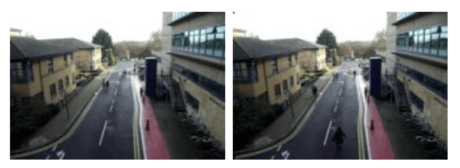
Figure 2.14 Sample frames from the test video ‘can_220_street(1)’. [Video Courtesy of SULFA]

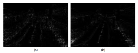
Figure 2.15 SPN patterns for (a) a single frame from the test video ‘can_220_street(1).mov’ and (b) entire test video, obtained using 2D median filter.

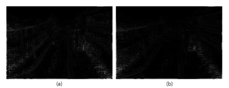
Figure 2.16 SPN patterns for (a) a single frame from the test video ‘can_220_street(1).mov’ and (b) entire test video, obtained using 2D Wiener filter.

As is evident from these results, the amount of scene details present in the SPN is dependent on the choice of the denoising filter used during its estimation.

As a forensic feature, SPN is highly robust and efficacious. Not only does it vary from camera to camera but also follows a consistent pattern over every frame recorded by a particular camera. It is evenly distributed across every pixel of the frame, and therefore survives harsh compression. SPN also remains unaffected by environmental conditions such as temperature and humidity.

Please note that in the digital video forensics literature, PRNU and FPN are sometimes collectively referred to as SPN. Moreover, sometimes the terms PRNU and SPN are used interchangeably.

Blind Source Camera Identification

It was suggested in sub-section 1.6.2 in Chapter 1 that in case the source device is unavailable during forensic examination of a video, another video sequence recorded by the same device could be used to estimate the reference noise pattern for the source device. For instance, if the video under examination is a surveillance footage recorded by a certain CCTV camera (whose identity is known), and if that camera is unavailable at the time of investigation, then another video recorded by the same CCTV camera at some earlier point in time can be used to estimate reference PRNU or SPN. But for this to work, we must be absolutely certain that the video being used as reference was in fact, generated by the camera under consideration.

If we are uncertain of the identity of the recording device, or if no other video recorded by the same camera exists or is available, then the process of device linking becomes a little more complicated, because in this case, we need to train a machine-learning-based classification algorithm to categorize test noise patterns and infer the identity of the source camera in a blind manner.

A classification algorithm is a mathematical function that determines which of a set of categories a new observation belongs to. This determination is based on a training set of data, which contains observations (or instances) whose category membership is already known. A simple example of classification is categorizing a given email as ‘spam’ or ‘non-spam’. An algorithm that implements classification is known as a classifier. Some examples of commonly used classifiers are Support Vectors Machines (SVMs), k-Nearest Neighbors algorithm (k-NN), neural networks, naïve Bayes, and decision trees.

Blind source camera identification is performed in two steps:

Step 1 – Classifier Training: The first step is to train a classifier (the most frequently used classifier is an SMV). To train a classifier is to teach it to differentiate fingerprints of one acquisition device from those of another, and put different test images into different categories according to the fingerprints they exhibit. Training is performed with the help of certain distinguishing features, which are extracted from a training dataset consisting of numerous images and videos captured by a certain number of acquisition devices. The classifier is taught/trained to distinguish between images and videos acquired by different cameras based on the features exhibited by these images/videos.

Step 2 – Classifier Testing: Once the classifier is trained to categorize noise patterns into different classes (where each class represents an acquisition device), it is presented with a test video of unknown origin. The classifier analyzes the characteristics of noise patterns in the frames of this video, and based on the distinguishing features, tries to determine which device is most likely to have generated them. So it basically classifies the test data as belonging to one of the classes it was taught about during training.

Although recent innovations in the machine-learning domain have helped improve the accuracy of machine learning-based source identification schemes significantly, they still suffer from some operational limitations, the most prominent among which are the time and cost-intensive nature of such schemes, which due to practical constraints, restricts the classifier to be trained on a limited number of camera models, and thus limits the widespread real life applicability of these schemes.

Summary

In this chapter, we examined the domain of source camera identification in detail. The discussion included an overview of the basic video acquisition pipeline, analysis of the various forensic artifacts used as fingerprints for identification of source cameras and camera-models, and the primary concepts of blind source camera identification. In the next chapter, we will learn about the different active-non-blind methods of video content authentication.

[custom-related-posts title="Related Posts" none_text="None found" order_by="title" order="ASC"]

April 29, 2020